Land degradation and SDG 15.3.1

As part of the “2030 Agenda for Sustainable Development”, Sustainable Development Goal (SDG) 15 is to:

“Protect, restore and promote sustainable use of terrestrial ecosystems, sustainably manage forests, combat desertification, and halt and reverse land degradation and halt biodiversity loss”

Each SDG has specific targets addressing different components, in this case, of life on land. Target 15.3 aims to:

“By 2030, combat desertification, restore degraded land and soil, including land affected by desertification, drought and floods, and strive to achieve a land degradation-neutral world”

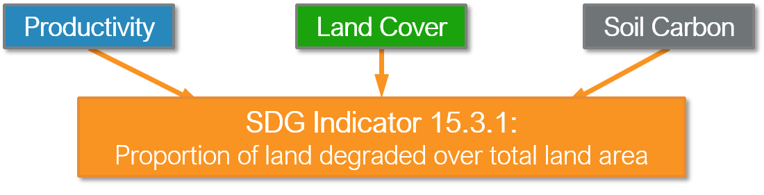
Indicators will be used then to assess the progress of each SDG target. In the case of SDG 15.3 the progress towards a land degradation neutral world will be assessed using indicator 15.3.1:

“proportion of land that is degraded over total land area”

As the custodian agency for SDG 15.3, the United Nations Convention to Combat Desertification (UNCCD) has developed a Good Practice Guidance (GPG) providing recommendations on how to calculate SDG Indicator 15.3.1.

This page provides a brief introduction to SDG Indicator 15.3.1 and describes how each indicator is calculated by .

In order to assess the area degraded, SDG Indicator 15.3.1 uses information from 3 sub-indicators:

1. Vegetation productivity

2. Land cover

3. Soil organic carbon

allows the user to compute each of these sub-indicators in a spatially explicit way generating raster maps which are then integrated into a final SDG indicator 15.3.1 map and produces a table result reporting areas potentially improved and degraded for the area of analysis.

Sub-indicators

Productivity

Land productivity is the biological productive capacity of the land, the source of all the food, fiber and fuel that sustains humans (United Nations Statistical Commission 2016). Net primary productivity (NPP) is the net amount of carbon assimilated after photosynthesis and autotrophic respiration over a given period of time (Clark et al. 2001) and is typically represented in units such as kg/ha/yr. NPP is a variable time consuming and costly to estimate, for that reason, we rely on remotely sensed information to derive indicators of NPP.

One of the most commonly used surrogates of NPP is the Normalized Difference Vegetation Index (NDVI), computed using information from the red and near- infrared wavelengths of the electromagnetic spectrum. In we make use of bi-weekly products from MODIS and AVHRR to compute annual integrals of NDVI (computed as the mean annual NDVI for simplicity of interpretation of results). These annual integrals of NDVI are then used to compute each of the productivity metrics explained below.

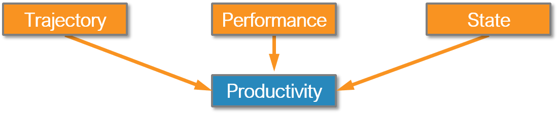
Land productivity is assessed in using three measures of change derived from NDVI time series data: trajectory, performance and state

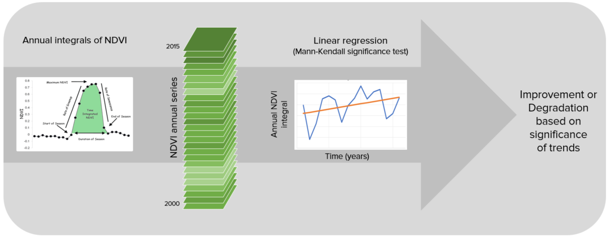
Productivity Trajectory

Trajectory measures the rate of change in primary productivity over time. As indicated in the figure below, computes a linear regression at the pixel level to identify areas experiencing changes in primary productivity for the period under analysis. A Mann-Kendall non-paremetric significance test is then applied, considering only significant changes those that show a p-value ≤ 0.05. Positive significant trends in NDVI would indicate potential improvement in land condition, and negative significant trends potential degradation.

Correcting for the effects of climate

Within a given ecosystem, primary productivity is affected by several factors, such as temperature, and the availability of light, nutrients and water. Of those, water availability is the most variable over time, and can have very significant influences in the amount of plant tissue produced every year. When annual integrals of NDVI are used to perform the trajectory analysis, it is important to interpret the results having historical precipitation information as a context. Otherwise, declining productivity trends could be identified as human caused land degradation, when they are driven by regional patterns of changes in water availability.

allows the user to perform different types of analysis to separate the climatic causes of the changes in primary productivity, from those which could be a consequence of human land use decisions on the ground. The methods currently supported for climate corrections are:

Residual Trend Analysis (RESTREND): RESTREND uses linear regression models to predict NDVI for a given rainfall amount. Trends in the difference between the predicted NDVI and the observed NDVI (the residual) are interpreted as non-climatically related productivity change. Please refer to the following citation more more details on the method and its limitations: Wessels, K.J.; van den Bergh, F.; Scholes, R.J. Limits to detectability of land degradation by trend analysis of vegetation index data. Remote Sens. Environ. 2012, 125, 10–22.

Rain Use Efficiency (RUE): RUE Is the ratio of annual NPP to annual precipitation. uses the annual integrals of NDVI as a proxy for annual NPP, and offers the possibility of choosing among different precipitation products to compute RUE. After RUE is computed for each of the years under analysis, a linear regression and a non-parametric significance test is applied to the trend of RUE over time. Positive significant trends in RUE would indicate potential improvement in land condition, and negative significant trends potential degradation. Please refer to the following publication for details on the methods and its limitations: Wessels, K.J.; Prince, S.D.; Malherbe, J.; Small, J.; Frost, P.E.; VanZyl, D. Can human-induced land degradation be distinguished from the effects of rainfall variability? A case study in South Africa. J. Arid Environ. 2007, 68, 271–297.

Water Use Efficiency (WUE): RUE assumes that there is a linear relationship between the amount of water that falls in the form of precipitation in a particular place and the amount of water which will be actually used by the plants. This assumption does not hold true for every system. WUE tries to address this limitation by using total annual evapo-transpiration (ET) instead precipitation. ET is defined as precipitation minus the water lost to surface runoff, recharge to groundwater and changes to soil water storage. The rest of the analysis follows as described for RUE: a linear regression and a non-parametric significance test is applied to the trend of WUE over time. Positive significant trends in WUE would indicate potential improvement in land condition, and negative significant trends potential degradation.

The table below list the datasets available in to perform NDVI trend analysis over time using the original NDVI data or with climatic corrections:

Variable	Sensor/Dataset	Temporal	Spatial Res.	Extent	Units/Description
NDVI	AVHRR/GIMMS	1982-2015	8 km	Global	Mean annual NDVI * 10000
NDVI	MOD13Q1-coll6.1	2001-2024	250 m	Global	Mean annual NDVI * 10000
Soil moisture	MERRA 2	1980-2019	0.5° x 0.625°	Global	Water root zone m3m-3 *10000
Soil moisture	ERA I	1979-2016	0.75° x 0.75°	Global	Volumetric Soil Water layer m3m-3 (0-7 cm)
Precipitation	GPCP v2.3.1 monthly (Global Precipitation Climatology Project)	1979-2019	2.5° x 2.5°	Global	mm/year
Precipitation	GPCC V6 (Global Precipitation Climatology Centre)	1891-2019	1° x 1°	Global	mm/year
Precipitation	CHIRPS	1981-2024	5 km	50°N x 50°S	mm/year
Precipitation	PERSIANN-CDR	1983-2024	25 km	60°N x 60°S	mm/year
Evapotranspiration	MOD16A2.GF	2000-2024	500 m	Global	Annual ET kg/m2 (=mm)*10

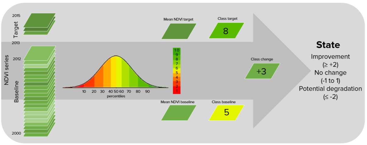
Productivity State

The Productivity State metric allows for the detection of recent changes in primary productivity as compared to a baseline period. The State metric is computed as follows:

1. Define the baseline period (historical period to which to compare recent primary productivity).

2. Define the comparison period (recent years used to compute comparison). It is recommended to use a 3-year to avoid annual fluctuations related to climate.

3. For each pixel, use the annual integrals of NDVI for the baseline period to compute a frequency distribution. In case the baseline period missed some extreme values in NDVI, add 5% on both extremes of the distribution. That expanded frequency distribution curve is then used to define the cut-off values of the 10 percentile classes.

4. Compute the mean NDVI for the baseline period, and determine the percentile class it belongs to. Assign to the mean NDVI for the baseline period the number corresponding to that percentile class. Possible values range from 1 (lowest class) to 10 (highest class).

5. Compute the mean NDVI for the comparison period, and determine the percentile class it belongs to. Assign to the mean NDVI for the comparison period the number corresponding to that percentile class. Possible values range from 1 (lowest class) to 10 (highest class).

6. Determine the difference in class number between the comparison and the baseline period (comparison minus baseline).

7. If the difference in class between the baseline and the comparison period is ≤ 2, then that pixel could potentially be degraded. If the difference is ≥ 2, that pixel would indicate a recent improvement in terms of primary productivity. Pixels with small changes are considered stable.

The table below list the datasets available in to compute the Productivity State metric:

Variable	Sensor/Dataset	Temporal	Spatial Res.	Extent	Units/Description
NDVI	AVHRR/GIMMS	1982-2015	8 km	Global	Mean annual NDVI * 10000
NDVI	MOD13Q1-coll6.1	2001-2024	250 m	Global	Mean annual NDVI * 10000

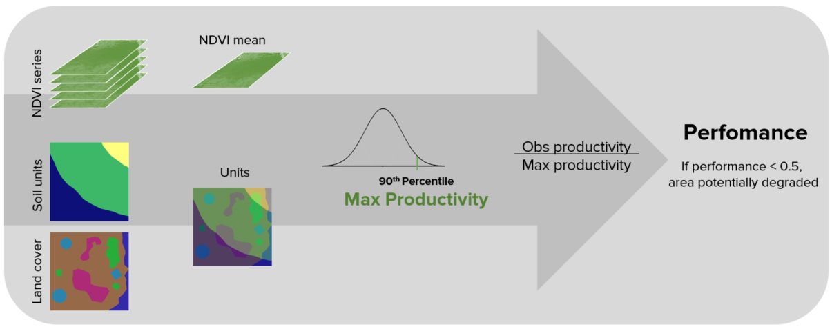
Productivity Performance

The Productivity Performance metric measures local productivity relative to other similar vegetation types in similar land cover types or bioclimatic regions throughout the study area. uses the unique combination of soil units (soil taxonomy units using USDA system provided by SoilGrids at 250m resolution) and land cover (full 37 land cover classes provided by ESA CCI at 300m resolution) to define this areas of analysis. The Performance metric is computed as follows:

1. Define the analysis period, and use the time series of NDVI to compute mean the NDVI for each pixel.

2. Define similar ecologically similar units as the unique intersection of land cover and soil type.

3. For each unit, extract all the mean NDVI values computed in step 1, and create a frequency distribution. From this distribution determine the value which represents the 90th percentile (we don’t recommend using the absolute maximum NDVI value to avoid possible errors due to the presence of outliers). The value representing the 90th percentile will be considered the maximum productivity for that unit.

4. Compute the ratio of mean NDVI and maximum productivity (in each case compare the mean observed value to the maximum for its corresponding unit).

5. If observed mean NDVI is lower than 50% than the maximum productivity, that pixel is considered potentially degraded for this metric.

The table below list the datasets available in to compute the Productivity Performance metric:

Variable	Sensor/Dataset	Temporal	Spatial Res.	Extent	Units/Description
NDVI	AVHRR/GIMMS	1982-2015	8 km	Global	Mean annual NDVI * 10000
NDVI	MOD13Q1-coll6.1	2001-2024	250 m	Global	Mean annual NDVI * 10000
Land Cover	ESA CCI	1992-2022	300 m	Global	Land cover thematic classes
Soil taxonomic units	SoilGrids - USDA	Static	250 m	Global	Soil units

Combining Productivity Metrics

The three productivity metrics are then combined as indicated in the tables below. For SDG 15.3.1 reporting, the 3-class indicator is required, but also produces a 5-class one which takes advantage of the information provided by State to inform the type of degradation occurring in the area.

Aggregating Land Productivity metrics

Trend	State	Performance
Improving	Improving	Stable
Improving	Improving	Degrading
Improving	Stable	Stable
Improving	Stable	Degrading
Improving	Degrading	Stable
Improving	Degrading	Degrading
Stable	Improving	Stable
Stable	Improving	Degrading
Stable	Stable	Stable
Stable	Stable	Degrading
Stable	Degrading	Stable
Stable	Degrading	Degrading
Degrading	Improving	Stable
Degrading	Improving	Degrading
Degrading	Stable	Stable
Degrading	Stable	Degrading
Degrading	Degrading	Stable
Degrading	Degrading	Degrading

➡

5 Classes	3 Classes
Improving	Improving
Improving	Improving
Improving	Improving
Improving	Improving
Improving	Improving
Moderate decline	Degrading
Stable	Stable
Stable	Stable
Stable	Stable
Stressed	Stable
Moderate decline	Degrading
Degrading	Degrading
Degrading	Degrading
Degrading	Degrading
Degrading	Degrading
Degrading	Degrading
Degrading	Degrading
Degrading	Degrading

Land cover

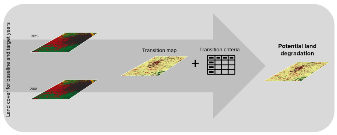
To assess changes in land cover users need land cover maps covering the study area for the baseline and target years. These maps need to be of acceptable accuracy and created in such a way which allows for valid comparisons. uses ESA CCI land cover maps as the default dataset, but local maps can also be used. The indicator is computed as follows:

1. Reclassify both land cover maps to the 7 land cover classes needed for reporting to the UNCCD (forest, grassland, cropland, wetland, artificial area, bare land and water).

2. Perform a land cover transition analysis to identify which pixels remained in the same land cover class, and which ones changed.

3. Based on your local knowledge of the conditions in the study area and the land degradation processed occurring there, use the table below to identify which transitions correspond to degradation (- sign), improvement (+ sign), or no change in terms of land condition (zero).

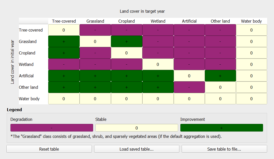
1. will combine the information from the land cover maps and the table of degradation typologies by land cover transition to compute the land cover sub-indicator.

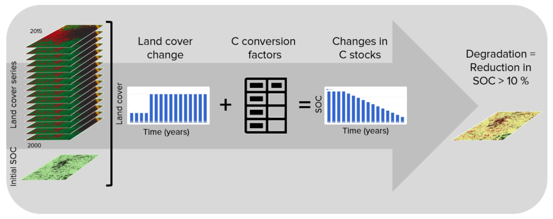
Soil organic carbon

The third sub-indicator for monitoring land degradation as part of the SDG process quantifies changes in soil organic carbon (SOC) over the reporting period. Changes in SOC are particularly difficult to assess for several reasons, some of them being the high spatial variability of soil properties, the time and cost intensiveness of conducting representative soil surveys and the lack of time series data on SOC for most regions of the world. To address some of the limitations, a combined land cover/SOC method is used in to estimate changes in SOC and identify potentially degraded areas. The indicator is computed as follows:

1. Determine the SOC reference values. uses SoilGrids 250m carbon stocks for the first 30 cm of the soil profile as the reference values for calculation (NOTE: SoilGrids uses information from a variety of data sources and ranging from many years to produce this product, therefore assigning a date for calculations purposes could cause inaccuracies in the stock change calculations).

2. Reclassify the land cover maps to the 7 land cover classes needed for reporting to the UNCCD (forest, grassland, cropland, wetland, artificial area, bare land and water). Ideally annual land cover maps are preferred, but at least land cover maps for the starting and end years are needed.

3. To estimate the changes in C stocks for the reporting period C conversion coefficients for changes in land use, management and inputs are recommended by the IPCC and the UNCCD. However, spatially explicit information on management and C inputs is not available for most regions. As such, only land use conversion coefficient can be applied for estimating changes in C stocks (using land cover as a proxy for land use). The coefficients used were the result of a literature review performed by the UNCCD and are presented in the table below. Those coefficients represent the proportional in C stocks after 20 years of land cover change.

LU coefficients	Forest	Grasslands	Croplands	Wetlands	Artificial areas	Bare lands	Water bodies
Forest	1	1	f	1	0.1	0.1	1
Grasslands	1	1	f	1	0.1	0.1	1
Croplands	1/f	1/f	1	1/0.71	0.1	0.1	1
Wetlands	1	1	0.71	1	0.1	0.1	1
Artificial areas	2	2	2	2	1	1	1
Bare lands	2	2	2	2	1	1	1
Water bodies	1	1	1	1	1	1	1

Changes in SOC are better studied for land cover transitions involving agriculture, and for that reason there is a different set of coefficients for each of the main global climatic regions: Temperate Dry (f = 0.80), Temperate Moist (f = 0.69), Tropical Dry (f = 0.58), Tropical Moist (f = 0.48), and Tropical Montane (f = 0.64).

4. Compute relative different in SOC between the baseline and the target period, areas which experienced a loss in SOC of 10% of more during the reporting period will be considered potentially degraded, and areas experiencing a gain of 10% or more as potentially improved.

Combining indicators into SDG Indicator 15.3.1

The integration of the three SDG 15.3.1 sub-indicators is done following the one-out all-out rule(1OAO), this means that if an area/pixel was identified as potentially degraded by any of the sub-indicators, then that area/pixel will be considered potentially degraded for reporting purposes.

Aggregating SDG 15.3.1 sub-indicators - 1OAO

Land Productivity	Land Cover	SOC
Improving	Improving	Improving
Improving	Improving	Stable
Improving	Improving	Declining
Improving	Stable	Improving
Improving	Stable	Stable
Improving	Stable	Declining
Improving	Declining	Improving
Improving	Declining	Stable
Improving	Declining	Declining
Stable	Improving	Improving
Stable	Improving	Stable
Stable	Improving	Declining
Stable	Stable	Improving
Stable	Stable	Stable
Stable	Stable	Declining
Stable	Declining	Improving
Stable	Declining	Stable
Stable	Declining	Declining
Declining	Improving	Improving
Declining	Improving	Stable
Declining	Improving	Declining
Declining	Stable	Improving
Declining	Stable	Stable
Declining	Stable	Declining
Declining	Declining	Improving
Declining	Declining	Stable
Declining	Declining	Declining

➡

SDG 15.3.1
Improving
Improving
Declining
Improving
Improving
Declining
Declining
Declining
Declining
Improving
Improving
Declining
Improving
Stable
Declining
Declining
Declining
Declining
Declining
Declining
Declining
Declining
Declining
Declining
Declining
Declining
Declining

Calculating Status map

According to the Good Practice Guidance Addendum SDG Indicator 15.3.1, the Status map “refers to the final condition (considering the baseline) of land at the end of each reporting period, classified as either degraded, stable, or improved”. It combines the SDG Indicator 15.3.1 layer calculated for a given period of assessment with the Baseline SDG Indicator 15.3.1. By combining these two layers, the Status map shows changes that happened over the period assessment integrated with land conditions (degradation, stabilily, improvement) mapped at the Baseline period, providing a more complete understanding of the land condition trajectory over time.

Note

The Status layer for the Baseline period is equivalent the SDG Indicator 15.3.1 calculated for the Baseline assessment (i.e. Baseline Assessment == Status 2015).

For combining a given period assessment with the Baseline SDG Indicator 15.3.1 it is necessary to apply the 3 x 3 Status Matrix

		PERIOD ASSESSMENT
		DEGRADED	STABLE*	IMPROVED*
BASELINE	DEGRADED	Degraded	Degraded	Improved
	STABLE*	Degraded	Stable	Improved
	IMPROVED*	Degraded	Improved	Improved

* Not Degraded areas.

Note

For further information on how to derive the Status map, please refer to the Good Practice Guidance Addendum SDG Indicator 15.3.1 which offers a dedicated section on “Assessing Status for each reporting process” starting on page 19.

Expanded Status Matrix

While the status map resulting from the above comparison provides a snapshot of land condition at the end of the reporting period in three broad categories (Degraded, Stable, and Improved), the underlying dynamics that lead to this final status can be complex - there are nine different types of changes (given it is a 3x3 matrix) in land condition. Understanding these different pathways enables a deeper interpretation of the land condition changes, allowing for the identification of gains and losses of natural capital that have occurred relative to a baseline state. For example, degradation and improvement can correspond to recent changes, a continuation of ongoing trends in areas previously degraded or improved, or stability in areas that were already degraded or improved in a prior period.

The below status matrix can be used instead of the 3x3 matrix above to capture these different types of changes in land condition that can occur. This expanded version of the status matrix allows for a more detailed classification of land condition changes, providing insights into the nature and timing of degradation and improvement processes.

		PERIOD ASSESSMENT
		DEGRADED	STABLE	IMPROVED
BASELINE	DEGRADED	1 - Persistent Degradation	3 - Baseline Degradation	6 - Recent Improvement
	STABLE	2 - Recent Degradation	4 - Stability	6 - Recent Improvement
	IMPROVED	2 - Recent Degradation	5 - Baseline Improvement	7 - Persistent Improvement

Expanded version of the "Status Matrix" showing land condition that results from the comparison of the baseline (rows) and the period assessment (columns): degraded (purple), stable (yellow), and improved (green).

Each type of change represented in the expanded Status Matrix is detailed below. The table captures the nine possible combinations in the 3 × 3 matrix, reflecting transitions from the baseline assessment to the current period assessment. For each combination, a brief interpretation of the change is provided, along with its classification as either a recent or baseline improvement or degradation. This classification helps in understanding whether the observed changes represent new developments that have occurred during the current reporting period or whether no changes in status have taken place.

Note

For further information on how to derive the expanded status map, please refer to the Good Practice Guidance Addendum SDG Indicator 15.3.1 which offers a dedicated section on “Further characterization of land degradation and improvement” starting on page 29.

UNCCD Strategic Objective 2 (SO 2)

To improve the living conditions of affected populations

Addressing the global challenges of desertification, land degradation, and drought (DLDD) and their impacts on coupled human-environmental systems is a key component of the 2030 Agenda for Sustainable Development. In particular, Sustainable Development Goal (SDG) 15.3 aims to, by 2030, combat desertification, restore degraded land and soil, including land affected by desertification, drought and floods, and strive to achieve a land degradation-neutral world. Addressing this challenge is essential for improving the livelihoods of those most affected by DLDD and for safeguarding against the most extreme effects of climate change.

The livelihoods of people in degraded areas include multiple human and natural characteristics of local environments, including adequate access to food and water, either directly through subsistence livelihoods, through sufficient income to purchase food and water security, or a combination of both. If food and water security are achieved, outmigration from affected areas should no longer be forced but rather voluntary in nature. Socially and economically marginalized populations, communities and households tend to be disproportionally vulnerable to climate change and the combined effects of DLDD. The ability to identify and quantify the makeup, distribution, and relative vulnerability of such populations,communities, and households is critical in reinforcing livelihood resilience in order to enhance positive adaptations to DLDD

How population exposure is calculated

allows users to monitor UNCCD’s Strategic Objective 2 indicator on Trends in Population Exposure to Land Degradation Disaggregated by Sex (SO 2-3) by calculating the proportions of population, disaggregated by sex, exposed to land degradation. uses gridded data representing the spatial distribution of the population over the SDG 15.3.1 Indicator map to establish its exposure to land degradation.

The (SO 2-3) indicator uses the following metrics:

• Percentage of the female population exposed to land degradation

• Percentage of the male population exposed to land degradation

• Percentage of the total (female and male) population exposed to land degradation

To calculate the SO 2-3 indicator, uses gridded population data from the WorldPop project. WorldPop provides separate raster layers for male and female population, each representing the estimated number of people per grid cell for a given year. overlays these population grids with the final SDG 15.3.1 indicator map, which classifies every pixel as degraded, stable, or improved. For each degradation class the tool sums the number of people — separately for males and females — whose grid cell falls within that class. Areas classified as water bodies are masked out and excluded from the totals, in line with UNCCD reporting requirements.

The resulting totals are then expressed as percentages of the total population within the area of interest, producing the three SO 2-3 metrics: the percentage of the female population, the male population, and the combined population exposed to land degradation. In the output map, pixels in degraded areas retain their population count as a positive value, pixels in improved areas are shown as negative values (indicating population in areas where conditions have improved), and water areas are marked as no-data. This sign convention makes it straightforward to distinguish, at a glance, populations living on degraded land from those on improving land.

UNCCD Strategic Objective 3 (SO 3)

To mitigate, adapt to, and manage the effects of drought in order to enhance resilience of vulnerable populations and ecosystems.

Drought and land degradation

Land degradation as defined by the UNCCD refers to any reduction or loss in the biological or economic productive capacity of the land resource base. It is generally caused by human activities, exacerbated by natural processes, and often magnified by and closely intertwined with climate change and biodiversity loss.Land degradation reduces agricultural productivity and increases the vulnerability of those areas already at risk of impacts from climate variability and change, especially in regions of the world.

Drought is a complex, slow-onset phenomenon that happens over different time scales. It is characterized by a reduction in water availability, leading to cascading effects on people’s livelihoods and economic sectors. Drought is sometimes simplistically defined as a period of dry weather long enough to cause a hydrological imbalance, although a globally agreed upon definition for drought does not exist. Moreover, drought hardly occurs as a single risk event but rather interlinked with other hazards such as heatwaves, wildfires, sand/dust storms, or floods.

The International Panel on Climate Change (IPCC) defines drought as “a period of abnormally dry weather long enough to cause a serious hydrological imbalance”. Drought is a relative term, therefore any discussion in terms of precipitation deficit must refer to the particular precipitation-related activity that is under discussion. For example, shortage of precipitation during the growing season impinges on crop production or ecosystem function in general (due to soil moisture drought, also termed agricultural drought), and during the runoff and percolation season primarily affects water supplies (hydrological drought). Storage changes in soil moisture and groundwater are also affected by increases in actual evapotranspiration in addition to reductions in precipitation. A period with an abnormal precipitation deficit is defined as a meteorological drought. See also Soil moisture (IPCC Assessment Report 5, 2014). The United Nations Disasters Risk Reduction (UNDRR) defines drought as a slow-onset hazard, often referred to as a creeping phenomenon. The absence of a precise, universally accepted definition of drought adds to the confusion. Definitions must be region specific because each climate regime has distinctive climatic characteristics (UNDRR GAR Chapter 6). The lack of agreed upon definition complicates monitoring efforts, as the definition and monitoring approach are typically context specific. where poverty rates remain high despite efforts to reduce poverty, inequality, and enhance the socio-economic well-being of all people worldwide.

Drought increasingly impacts larger numbers of people, livelihoods, ecosystems, and economies worldwide. When it occurs concomitantly with land degradation, it can expose already vulnerable populations to deleterious livelihood, environmental, socio-economic, and health risks and decrease population and community resilience.

The UNCCD has adopted a monitoring framework with three levels for SO 3:

Level I SO 3-1 Trends in the proportion of land under drought over the total land area(Hazard), Level II SO 3-2 Trends in the proportion of the total population exposed to drought(Exposure), Level III SO 3-3 Trends in the degree of drought vulnerability (Vulnerability).

Under the IPCC framework:

Hazard is the potential occurrence of a natural or human-induced physical event or trend or physical impact that may cause loss of life, injury, or other health impacts, as well as damage and loss to property, infrastructure, livelihoods, service provision, ecosystems and environmental resources.

Exposure characterizes the presence of people, livelihoods, species or ecosystems, environmental functions, services, and resources, infrastructure, or economic, social, or cultural assets in places and settings that could be adversely affected.

Vulnerability is defined as the propensity or predisposition to be adversely affected by climate change and related processes.

In order to assess the SO 3 indicators, uses information from 3 sub-indicators:

• Standardized Precipitation Index (SPI), alternatively the Standardized Precipitation Evapotranspiration Index (SPEI)

• Gridded global population dataset

• Drought Vulnerability Index (DVI)

allows the user to compute each of these indicators in a spatially explicit way generating raster maps and producing a summary table reporting areas potentially improved and degraded for the area of analysis. SO 3-1 “Trends in the proportion of land under drought over the total land area”.

The United Nations Convention to Combat Desertification (UNCCD) has developed a Good practice guidance for national reporting on UNCCD Strategic Objective 3 (GPG-SO3). providing recommendations on how to calculate indicators of SO3.

This document provides a brief introduction to the UNCCD Strategic Objective 3 and describes how each indicator is calculated by , following the Strategic Objective 3 Good Practice Guidance.

SO3 Level I indicator (SO 3-1 Hazard)

Steps to calculate Level I indicator following the UNCCD GPG-SO3:

1. Calculate SPI using an accumulation period of 12 months (SPI-12) and gridded precipitation data

2. Identify the drought intensity class of each pixel based on the previously calculated SPI

3. Calculate proportion of land within each drought intensity class.

Standardized Precipitation Index (SPI)

The Standardized Precipitation Index (SPI) has been widely used to characterize meteorological drought or precipitation deficit, and was recognized through the Lincoln Declaration on Drought as the internationally preferred index for calculating and monitoring meteorological drought. SPI is calculated as standard deviations that the observed precipitation over a specified period would deviate from the long-term mean over periods of that duration considered over typically 30 years of data, for a normal distribution and fitted probability distribution for the actual precipitation record. The primary advantages for using the SPI for global drought monitoring, prediction, and risk assessment is that it is currently in use in many countries globally and is endorsed by the World Meteorological Organization. Other key advantages are that the SPI represents both precipitation deficits and surpluses, and it can be calculated at different timescales (e.g., SPI-3, SPI-6, SPI-12, with the number indicating the number of months over which the index is calculated). Thus, it indirectly considers effects of accumulating precipitation deficits, which are critical for soil moisture and hydrological droughts.

By default, offers access to SPI calculated from the Global Precipitation Climatology Centre (GPCC) Monitoring Product, a raster representing precipitation and derived from rain gauge data featuring spatial resolution of ~27 sq km and covering the entire globe. Users have also the option to use an alternative SPI calculated from the Climate Hazards Group InfraRed Precipitation with Stations (CHIRPS), with precipitation estimates based on satellite observations combined to gauged station data at ~5 sq km. While CHIRPS features higher spatial resolution, it has a “quasi-global” coverage that spans 50°S to 50°N. Therefore, users interested in calculating SO3-1 Hazard for areas outside this range will not be able to use the CHRIPS dataset.

Step 1. Calculating SPI

The SPI quantifies observed precipitation as a standardized departure from a selected probability distribution function that models the raw data. The raw data can be fitted to a gamma or a Pearson Type III distribution, and then transformed to a normal distribution. The transformed precipitation data are then used to compute the dimensionless SPI value, defined as the standardized anomaly of the precipitation.

The detailed equations for computing this index are described in the following steps using the gamma distribution:

1. The transformation of the precipitation value into SPI has the purpose of:

   1. Transforming the mean of the precipitation value adjusted to 0;

   2. Standard deviation of the precipitation is adjusted to 1.0; and

   3. Skewness of the existing data must be readjusted to zero.

When these goals have been achieved the standardized precipitation index can be interpreted as mean 0 and standard deviation of 1.0.

2. Mean of the precipitation can be computed as:

where N is the number of precipitation observations.

3. The standard deviation for the precipitation is computed as:

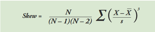
4. The skewness of the given precipitation is computed as:

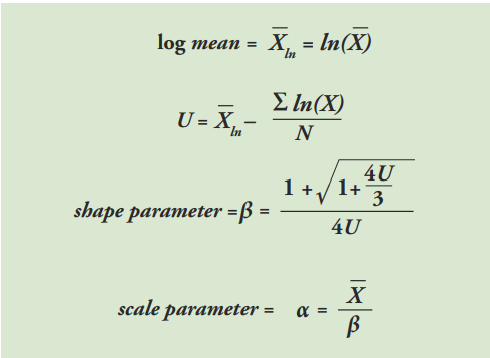
5. The precipitation is converted to lognormal values and the statistics U, shape and scale parameters of gamma distribution is computed:

6. The resulting parameters are then used to find the cumulative probability of an observed precipitation event. The cumulative probability is given by:

7. Since the gamma function is undefined for x = 0 and a precipitation distribution may contain zeros, the cumulative probability becomes:

where the probability from q is zero.

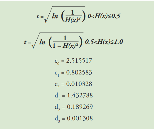
8. The cumulative probability H(x) is then transformed to the standard normal random variable Z with mean zero and variance of one:

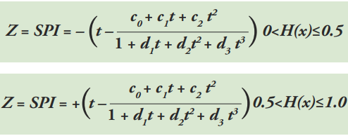
where:

Step 2. Identifying drought intensity classes

The dimensionless SPI values are interpreted as the number of standard deviations by which the observed anomaly deviates from the long-term mean and are typically labeled categorically based on condition (i.e., extremely wet, extremely dry, normal) as shown in the table below. A drought occurs when the SPI is consecutively negative, and its value reaches an intensity of -1 or less and ends when the SPI becomes positive.

Description	Precipitation Category
2.0 or more	Extremely wet
1.5 to 1.99	Severely wet
1.0 to 1.49	Moderately wet
-0.99 to 0.99	Near normal
-1.0 to -1.49	Moderately dry
-1.5 to -1.99	Severely dry
-2.0 or less	Extremely dry

Drought intensity classes are identified by assessing the December SPI-12 values for ear year of time-series. The December SPI-12 values represent the precipitation deficits (or excesses) over the Gregorian (January-December) calendar year. Positive SPI values are discarded, since they indicate that there was no drought in the given period.

For further details on SPI, see the Good practice guidance for national reporting on UNCCD Strategic Objective 3. We also recommend reading the Tools4LDN Technical Report on Monitoring Progress Towards UNCCD Strategic Objective 3 A review of Publicly Available Geospatial Datasets and Indicators in Support of Drought Monitoring.

Step 3. Calculating the proportion of land within each drought intensity class.

The equation to estimate the percentage of land within drought intensity classes takes the land area under the each drought intensity class identified in the previous step over the the total land area, as follows:

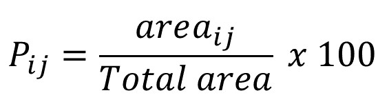
Where:

Pij is the proportion of land under the drought intensity class i in the year j

areaij is the land area under the drought intensity class i in the reporting year j

Total area is all the total land area.

SO3 Level II indicator (SO 3-2 Exposure)

The UNCCD SO3 Level III drought Exposure indicator is built upon the SO 3 Level I Hazard indicator by overlaying a gridded population data. Using the overlaying population as a proxy for calculating drought exposure is a straight-forward method. Knowing how many people are directly affected by drought can help aid get allocated to the most needed areas, based on percent of population exposed and strength of that exposure (drought severity). This method can also serve as a proxy for socioeconomic drought.The gender disaggregation calculation for the SO3 Level II population indicator is computed based on percent male and percent female in each grid cell. The outputs include exposure information by gender (percent male and percent female) exposed to each Level I drought intensity class. This produces two comparable grids that could be aggregated to administrative boundaries if desired, where global and local spatial relationships between gender and drought occurrence and/or severity can be better quantified and visualized.

The WorldPop collection is a global gridded high resolution geospatial dataset on population distributions,demographics, and dynamics. WorldPop’s spatially disaggregated layers are gridded with an output resolution of 3 arc-seconds and 30 arc-seconds (approximately 100 m & 1 km, respectively at the equator) and incorporates inputs such as population census tables & national geographic boundaries, roads, land cover, built structures, urban areas, night-time lights, infrastructure, environmental data, protected areas, and water bodies. The strengths of WorldPop are that the population estimation method of dasymetric mapping is multivariate, i.e., highly modeled, and therefore tailored to match data conditions and geographical nature of each individual country and region. Gender information is also available. The weakness of WorldPop is that the utilization of such complex interpolation models with sparse census data may lead to highly uncertain and imprecise population estimates in some sub-national and rural regions. In spite of the aforementioned limitation, WorldPop remains the most ideal gridded population dataset as it satisfies all our inclusion criteria, including spatial resolution, global coverage, frequency of data updates, and inclusion of a gender-disaggregated component.

The percentages of population Exposure to drought are calculated by the number of people within each drought intensity classes over of the total population.

How population exposure to drought is represented in Trends.Earth

The SO 3-2 Exposure summary output in Trends.Earth is a multi-band raster file. Bands are organised in pairs, one pair per drought reporting period (each period is by default 4 years). Within each pair:

• The first band contains the most severe SPI value recorded during that period — the minimum SPI across all years in the period. A negative SPI indicates a precipitation deficit relative to the long-term mean, i.e., drought conditions.

• The second band contains the population count for the pixel at the time of the most severe drought, with the sign of the value encoding drought exposure:

  • A negative population value indicates that the pixel experienced drought during that period (minimum SPI < 0).

  • A positive population value indicates that the pixel experienced above-average precipitation during that period (SPI ≥ 0 throughout the entire period).

  • Pixels over water bodies are set to no-data, in line with UNCCD reporting requirements.

For the final drought period only, if sex-disaggregated population data are available, two additional bands follow the standard pair: a female population band and a male population band, both using the same sign convention described above.

This encoding makes it straightforward to derive exposure statistics from a single band: the absolute values of all valid pixels give the total population, while the absolute values of the negative pixels alone give the drought-exposed population.

SO3 Level III indicator (SO 3-3 Vulnerability)

Drought Vulnerability assessment is based on the Drought Vulnerability Index (DVI), a composite index incorporating three components reflecting the vulnerability of the population to drought: i) social, ii) economic and iii) infrastructural. Currently DVI does not feature components on ecological or ecosystem vulnerability. offers access to the global default DVI dataset produced by the Joint Research Centre (JRC). The JRC has developed a framework which integrates 15 economic, social, and infrastructural components related to drought vulnerability derived from global data sources. This framework recommends that drought vulnerability indicators should encompass orthogonal social, infrastructural, and economic factors that are generic and valid for any region.

The JRC framework for monitoring drought risk as described in Carrão et al., 2016 adopts an approach for SO3 assessing drought vulnerability that was initially proposed by the United Nations Office for Disaster Risk Reduction (UNDRR - formerly the United Nations International Strategy for Disaster Reduction or UNISDR) that reflects the state of the individual and collective social, economic, and infrastructural factors of a region [61]. This methodology has also been operationally implemented within the JRC Global Drought Observatory (GDO) to document and map global risk of drought impact for agriculture. The authors state that the factors that have been included do not represent a complete description of vulnerability in relation to a specific exposed element but can be viewed as the foundation for building a regional plan for reducing vulnerability and facilitating adaptation.

The methodology used in Carrão et al., 2016 follows the concept that individuals and populations require a range of semi-) independent factors characterized by a set of proxy indicators to achieve positive resilience to impacts. The methodology uses a two-step composite model that derives from the aggregation of 15 proxy indicators (show in the Table below) that represent social, economic, and infrastructural vulnerability at each geographic location (a similar methodology as the DVI, discussed subsequently) and are derived from both at the national level and very high spatial resolution gridded data.

Proxy indicators for vulnerability to drought used in Carrao et al. 2016 (Table 1). With the exception of gROADS and FAO’s Irrigated Agricultural Lands which are both gridded data, all data are available only at the national level. (Also draws on Table 14 from the Good practice guidance for national reporting on UNCCD Strategic Objective 3.)

Indicator	Source	Link
ECONOMIC
Energy consumption per capita (millions Btu per person)	US Energy Information Administration (U.S. EIA)	http://www.eia.gov/
Agriculture (% of GDP)	World Bank	http://data.worldbank.org/products/wdi
GDP per capita (current US$)	World Bank	http://data.worldbank.org/products/wdi
Poverty headcount ratio at $1.25 per day (PPP) (% of total population)	World Bank	http://data.worldbank.org/products/wdi
SOCIAL
Rural population (% of total population)	World Bank	http://data.worldbank.org/products/wdi
Literacy rate (% of people age 15 and above)	World Bank	http://data.worldbank.org/products/wdi
Improved water resources (% of rural population with access)	World Bank	http://data.worldbank.org/products/wdi
Life expectancy at birth (years)	World Bank	http://data.worldbank.org/products/wdi
Population ages 15-64 (% of total population)	World Bank	http://data.worldbank.org/products/wdi
Refugee population by country or territory of asylum (% of total population)	World Bank	http://data.worldbank.org/products/wdi
Government effectiveness	Worldwide Governance Indicators (WGI)	https://www.worldbank.org/en/publication/worldwide-governance-indicators/interactive-data-access
Disaster prevention & preparedness (US$/year/capita)	Organization for Economic Cooperation and Development (OECD)	http://stats.oecd.org/
INFRASTRUCTURAL
Agricultural and irrigated land (% of total agricultural land)	Food and Agricultural Administration (FAO)	http://www.fao.org/nr/water/aquastat/main/index.stm
% of retained renewable water	Aqueduct	http://www.wri.org/our-work/project/aqueduct
Road density (km of road per 100 sq.km. of land area)	gROADSv1	https://data.nasa.gov/dataset/global-roads-open-access-data-set-version-1-groadsv1

This process involves first combining the indicators presented in the Table for each factor using a Data Envelopment Analysis (DEA) model, a deterministic and non-parametric linear programming technique that can be used to quantify the relative exposure of a region to drought from a multidimensional set of indicators. Secondly, arithmetically aggregating the individual factors resulting from the DEA model into a composite model of drought vulnerability such that:

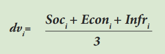
where Soc i, Econ i, and Infr i are the social, economic, and infrastructural vulnerability factors for region i.