Land Consumption and SDG 11.3.1
Background
Note
Source: UN-Habitat (2019) SDG Indicator 11.3.1 Training Module: Land Use Efficiency. United Nations Human Settlement Programme (UN-Habitat), Nairobi.
Human settlements, in all their diverse forms, appropriate land in varied ways. Just like living organisms, urban settlements (cities) evolve, transform, adapt, innovate and change with emerging trends. Urban settlements expand, shrink, densify, intensify, age, and sometimes their functions even migrate to areas that are more conducive to their survival. All these trends in urban settlements are closely associated with such factors as changes in population, economic potential and productivity, prevailing physical and social conditions, presence of enabling policies, among other things.
A country that maximizes the many benefits associated with urbanization is one that is able to understand, measure and predict the growth trends of its urban areas; and in turn put in place the necessary actions/interventions to tap on the benefits of such growth, while minimizing the equally diverse challenges associated with unplanned urbanization. Pro-active planning - which is a major pre-requisite for sustainable urbanization - requires that city authorities and other relevant actors predict the direction of growth of a city, and/or shape this growth by providing the required facilities, services and policy and legal frameworks ahead of development. This results in planned and equitable growth in which majority of the city residents have access to the basic services, economic and social opportunities, and where environmental sustainability prevails. At the center of all these is the need for generation and dissemination of up-to-date and accurate data on growth trends across cities and urban settlements.
Target 11.3 aims to enhance inclusive and sustainable urbanization and capacity for participatory, integrated and sustainable human settlement planning and management in all countries by 2030. To monitor progress towards the achievement of target 11.3 the UN established indicator 11.3.1, which measures how efficiently cities utilize land, which is measured as a ratio of the rate at which cities spatially consume land against the rate at which their populations grow. Empirical evidence has shown that, cities that are compact use land more efficiently and are better placed to provide public goods and basic services at a lower cost. Such cities can consume less energy, manage waste better, and are more likely to maximize the benefits associated with economics of agglomeration. On the other hand, sprawling cities (non-compact cities) experience increased demand for mobility; increased energy consumption; environmental degradation; increased cost of providing basic services per capita (e.g. water, sanitation, drainage); increased cost of infrastructure per capita; reduction in economies of agglomeration; and decreased urban productivity.
By measuring the rate at which cities consume land against their rate of population growth, city authorities and decision makers can project demand for public goods and services, identify new areas of growth, and pro-actively influence sustainable urban development. This is needed to provide adequate infrastructure, services and amenities for the improvement of living conditions to all. Generation and dissemination of data on this indicator is thus not only crucial for understanding urban growth dynamics and formulation of informed policies and guidelines, but is also at the core of promoting sustainable urbanization.
Rationale for Monitoring
Note
Source: UN-Habitat (2019) SDG Indicator 11.3.1 Training Module: Land Use Efficiency. United Nations Human Settlement Programme (UN-Habitat), Nairobi.
Understanding how a city/urban area expands spatially against its rate of population change is critical to determining, among other things, the nature of human settlements growth (formal versus informal) and the speed of conversion of outlying land to urbanized functions. These two elements have significant implications on the demand for and cost of providing services, as well as on environmental preservation and conservation.
To attain sustainable development, countries need to understand how fast their urban areas are growing, and in which direction. This will not only help them understand growth trends and effectively address demand for basic services but also help create policies that encourage optimal use of urban land, effectively protecting other land uses (natural environments, farmlands, etc). In addition, achievement of inclusive and sustainable urbanization requires that the resources be utilized in a manner that can accommodate population growth from migration and natural increase while preserving environmentally sensitive areas from development.
The purpose of monitoring progress against the SDG indicator 11.3.1 is therefore to provide necessary and timely information to decision makers and stakeholders in order to accelerate progress towards enhanced inclusive and sustainable urbanization. Meeting Target 11.3 by 2030 requires, at the minimum, slowing down urban sprawl and if possible, ensuring that the compactness of cities is maintained or increased over time.
Indicator and data needs
Indicator 11.3.1 is defined as the ratio of land consumption rate to population growth rate (Figure 1). In order to compute this indicator, information on the urban extent and population in at least two moments in time are needed, and even more if we are interested in assessing the change in the indicator over time.
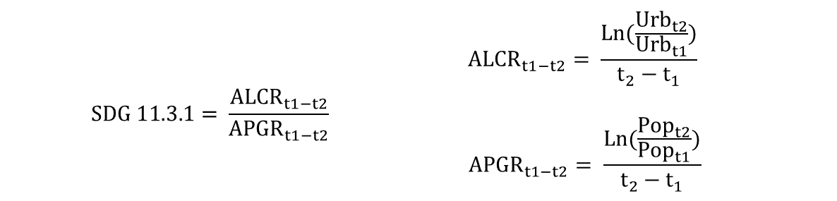
Figure 1: Sustainable development goal (SDG) indicator 11.3.1 is computed as the ratio of the annual land consumption rate (ALCR) to the annual population growth rate (APGR) between times 1 and 2. Ln: natural logarithm, Urb: urban area, pop: population, t: time in years.
Assessing changes in SDG 11.3.1. over time requires a significant amount of information, since it requires knowing urban extent and population count for multiple years. Earth observation data allow us to estimate the extent of built-up area within a city, and then using spatial analysis algorithms estimate the extent of the different elements within the urban environment (e.g. buildings, open space, water bodies, etc.). In ![]() we have adopted the work-flow below (Figure 2) to facilitate the process. Making use of Google Earth Engine’s super computers, the full Landsat archive between 1997 and 2019, and the GMIS dataset (Brown de Colstoun et al 2017),
we have adopted the work-flow below (Figure 2) to facilitate the process. Making use of Google Earth Engine’s super computers, the full Landsat archive between 1997 and 2019, and the GMIS dataset (Brown de Colstoun et al 2017), ![]() computed a series of impervious surface indices globally available at 30m resolution to inform on urban extent for the years 2000, 2005, 2010, and 2015. Combined with user input and population data, the tool computes SDG 11.3.1 both in the form of maps and tables for ease of interpretation and reporting.
computed a series of impervious surface indices globally available at 30m resolution to inform on urban extent for the years 2000, 2005, 2010, and 2015. Combined with user input and population data, the tool computes SDG 11.3.1 both in the form of maps and tables for ease of interpretation and reporting.
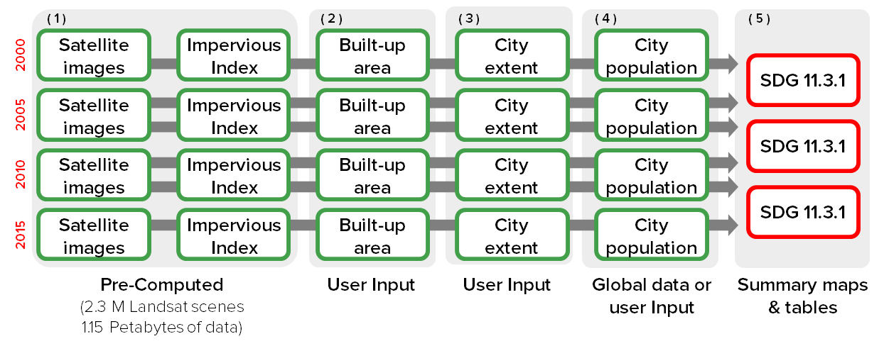
Figure 2: Trends.Earth works-flow to computing SDG 11.3.1. Global 30m impervious surface indices have been pre-computed and are available for the users to explore in the Trends.Earth Urban Mapper where the user defines built-up extent by simply assigning a series of thresholds.
Land consumption
To estimate land consumption in ![]() , a pre-computed time series of impervious surface indicators are available globally at 30 m resolution. In the section below, you will learn how the indicators were computed, and some recommendation how to use them to compute the indicator for SDG 11.3.1.
, a pre-computed time series of impervious surface indicators are available globally at 30 m resolution. In the section below, you will learn how the indicators were computed, and some recommendation how to use them to compute the indicator for SDG 11.3.1.
ISI in Trends.Earth
Given the lack of availability of a time series of impervious surface dataset at fine spatial resolution to capture urban changes globally, we computed one making use of the best impervious surface dataset available, the Global Man-made Impervious Surface for the year 2010 (GMIS, Brown de Colstoun et al 2017) to train a series of global random forest models (Breiman 2001) in Google Earth Engine (Gorelick et al 2017) making use of 2.3 million Landsat images (1.15 Peta-bytes of data) between the years 1997 and 2019. To make sure that the models were trained only with high quality data, we combined GMIS with ESA CCI land cover data for the year 2010 as indicated in Figure 3. This dataset allowed us to train random forest models, which where then applied to a set of 24 band stacks derived from Landsat surface reflectance data to generate impervious surface indicators for the years 1998, 2000, 2005, 2010, 2015, and 2018. A series of 846 models were run, one per eco region as defined by the RESOLVE dataset (Dinerstein et al 2017).
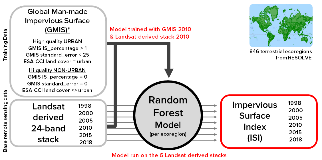
Figure 3: A series of 846 random forest models were run. Each model was trained using the GMIS and ESA CCI datasets, and then applied to a stack of 24 bands derived from Landsat imagery to predict impervious surface area for the years 1998, 2000, 2005, 2010, 2015, and 2018.
Since image availability is limited, in some areas, we included for each year images from the previous and posterior years (e.g. stack for 2005 includes images from 2004, 2005, and 2006). Each of the 24 band stacks contained the 7 reflectance bands (median for the 3 year period), 15 normalized difference indices representing all the possible combinations of the 7 original bands, and then 2 NDVI specific bands representing the maximum and the standard deviation of NDVI for each particular pixel during the 3-year period. Six of these stacks were generated for 1998, 2000, 2005, 2010, 2015, and 2018, and were the input to the random forest models.
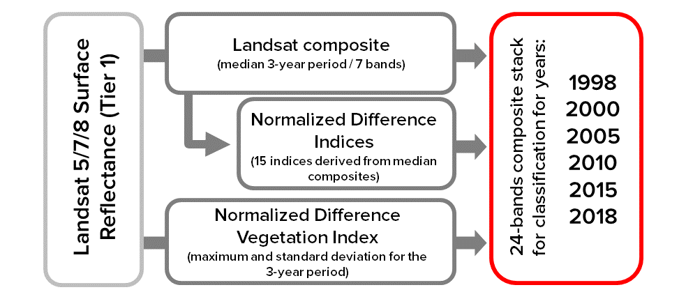
Figure 4: Description of the bands in the 24-band stack used in the random forest models.
It is hard to assess the accuracy of such dataset, given the lack of reference or comparable datasets globally. We compared the results of the 2010 ISI dataset to the GMIS original dataset for a subset of cities globally to assess its accuracy. We found that the root-mean-squared-error (RMSE) ranged between 9.9 and 14.4%, which for an indicator that varies between 0% (no impervious surface) to 100% (completely impervious), is a very acceptable result. We urge the users, however, to evaluate the results visually inspecting the Trends.Earth Urban Mapper for their area of interest.
From ISI to built-up
In order to estimate the area occupied by impervious surfaces in a city, we need to convert the continuous impervious surface index (ISI) into a binary map separating areas built from those not built. This process is done by defining a series of threshold values in the Trends.Earth Urban Mapper, which will vary by region.
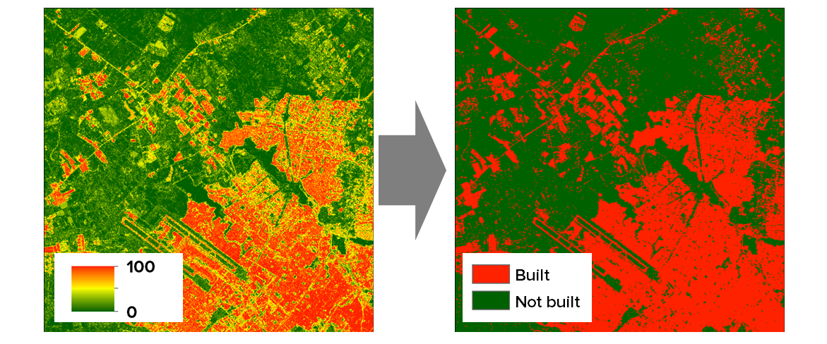
Figure 5: In Trends.Earth Urban Mapper the user has control on how the conversion from the continuous Impervious Surface Index (ISI, right) to the binary built up area map (built, left) will ocurr for their city of interest.
In ![]() the user needs to define 3 threshold values which will be used by the tool to estimate the built-up area for the area of interest. Those thresholds are:
the user needs to define 3 threshold values which will be used by the tool to estimate the built-up area for the area of interest. Those thresholds are:
Impervious Surface Index (ISI, 0-100): This is an index which varies between 0 and 100, with higher values being indicative of a higher percentage of impervious surface in the 30 m pixel. Setting the ISI threshold value lower will mean that your final built-up area dataset will include areas with low density of construction, usually found in the peripheries of the cities. Setting this value higher will make the assessment to focus on the high density city centers.
Night Time Lights Index (NTL, 0-100): The impervious surface index can, in some cases, present high values for areas covered with dry bare soil or rocks, since these type of surfaces have similar spectral properties as those of man-made impervious surfaces. To filter these areas we use night time lights, removing areas with high ISI and low night time lights present outside of city boundaries. The lack of a time series of night time lights of consistently calibrated for the time period considered (2000-2015), means that we can’t mask year with its corresponding year, so we use VIIRS Nighttime Day/Night Band Composites Version 1 for the year 2015 (NOA, 2019). Setting the NTL threshold value lower will mean that your final built-up area dataset will include areas with low light density, usually found in the peripheries of the cities. Setting this value higher will make the assessment to focus on the high density city centers.
Water Frequency Index (WFI, 0-100): Water presence is a very dynamic feature of coastal or riverine environment, in some cases water will inundate land areas, and in others, humans will encroach into water bodies to occupy the space. To capture some of those dynamics, we have integrated into the tool a water frequency dataset (Pekel et al 2016). By adjusting the water frequency threshold, the user can choose to highlight these land-water dynamic areas. Setting the water frequency threshold value lower will mean that your final built-up area dataset will consider as covered by water areas with lower water frequencies throughout the time series, such as intermittent rivers or lakes. Setting this value higher will restrict water bodies to areas with a high frequency of water occurrence (i.e. permanent rivers and lakes).
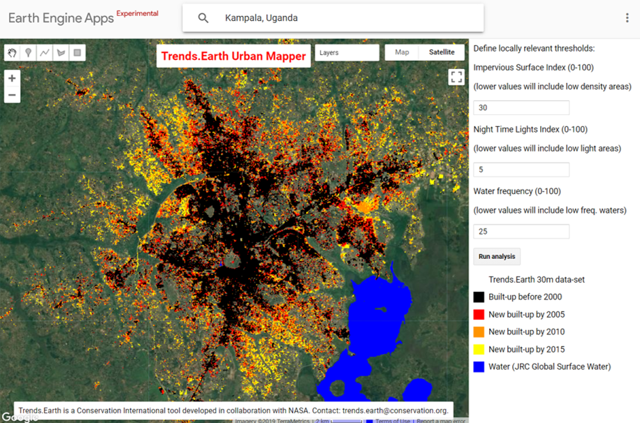
Figure 6: In Trends.Earth Urban Mapper the user defines a series of thresholds to go from the continuous Impervious Surface Index (ISI, right) to the binary built up area map (built, left).
Consistency test
When classifying remote sensing data into derived products, such as the impervious surface index computed by ![]() , omission and commission errors occur. One of the advantages of performing time series analysis is that the images from different years can be used to identify inconsistencies in the analysis. For that reason, 1998 and 2018 ISI layers were computed in this analysis, to add pre and post data points to filter possible errors in the classifications of the 2000 through 2015 series.
, omission and commission errors occur. One of the advantages of performing time series analysis is that the images from different years can be used to identify inconsistencies in the analysis. For that reason, 1998 and 2018 ISI layers were computed in this analysis, to add pre and post data points to filter possible errors in the classifications of the 2000 through 2015 series.
The thresholds defined in the previous section (ISI, NTL, and WFR) are applied to each of the individual layers of 1998, 2000, 2005, 2010, 2015, and 2018, generating a series of binary maps. The six binary maps are later combined into a time series dataset which contains information on the nature of each pixel for each year as “built-up” or “not-built”. One main rule is later applied to that series:
A pixel is considered built only if 50% or more of data points after the first built detection identify the same area as built. For such pixels, the first detection as built will be considered the year of conversion. Areas with less than 50% built after the first detection will be considered as errors in the classification, and as a consequence, not built. we recognize that by applying this rule we are limiting the capability of the dataset to detect transitions from built to not-built. However, given the low likelihood of that transition to occur in urban environments, we feel comfortable making that assumption. Visual inspection of the results support the approach.
Global testing
![]() provides through the Urban Mapper and the QGIS plug-in access to the global 30m time series of impervious surface indices. It is important however understand that the dataset has its limitations, and user’s input and control is needed to assess changes in indicator SDG 11.3.1 accurately. To test the performance of the indicator, we run the analysis on 224 cities globally (200 national capitals + 24 large cities in the Unites States of America, Figure 7). Using the Urban Mapper and visually comparing the product to very high spatial resolution images, we were able to define the thresholds appropriate for each city (ISI, NTL, and WFI) and also assess the quality of the product in a scale from 0 to 5. The results show that for 83% of the cities assessed Trends.Earth data can be used for estimating indicator SDG 11.3.1. The biggest limitation remains in small island states (for which no training data was available), hyper arid areas, and areas with low image availability.
provides through the Urban Mapper and the QGIS plug-in access to the global 30m time series of impervious surface indices. It is important however understand that the dataset has its limitations, and user’s input and control is needed to assess changes in indicator SDG 11.3.1 accurately. To test the performance of the indicator, we run the analysis on 224 cities globally (200 national capitals + 24 large cities in the Unites States of America, Figure 7). Using the Urban Mapper and visually comparing the product to very high spatial resolution images, we were able to define the thresholds appropriate for each city (ISI, NTL, and WFI) and also assess the quality of the product in a scale from 0 to 5. The results show that for 83% of the cities assessed Trends.Earth data can be used for estimating indicator SDG 11.3.1. The biggest limitation remains in small island states (for which no training data was available), hyper arid areas, and areas with low image availability.
No data: Cities for which no training data was available to build the impervious surface data set. These cities represent 6.2% of the sample assessed.
Unusable: Cities for which results are available, but due to low Landsat images availability prevented the production of a good quality product. These results should not be used for computing SDG 11.3.1 indicator. These cities represent 0.9% of the sample assessed.
Problematic: Cities with results of potential use for visually understating spatial patterns of built-up area expansion, but with significant errors. These results should not be used for computing SDG 11.3.1 indicator. These cities represent 4.0% of the sample assessed.
Some issues: Cities with results showing some issues confusing bare soil surfaces with built up area, could be used for computing SDG 11.3.1 after detailed inspection of the data. These cities represent 6.2% of the sample assessed.
Minor issues: Cities with high quality data but with the presence of some small areas of confusion. This data could be used for computing SDG 11.3.1. These cities represent 12.5% of the sample assessed.
High quality: Cities with high quality data showing perfect agreement between built-up area using Trends.Earth data and high resolution images available in Google Earth, high confidence for estimating SDG 11.3.1. These cities represent 70.1% of the sample assessed.
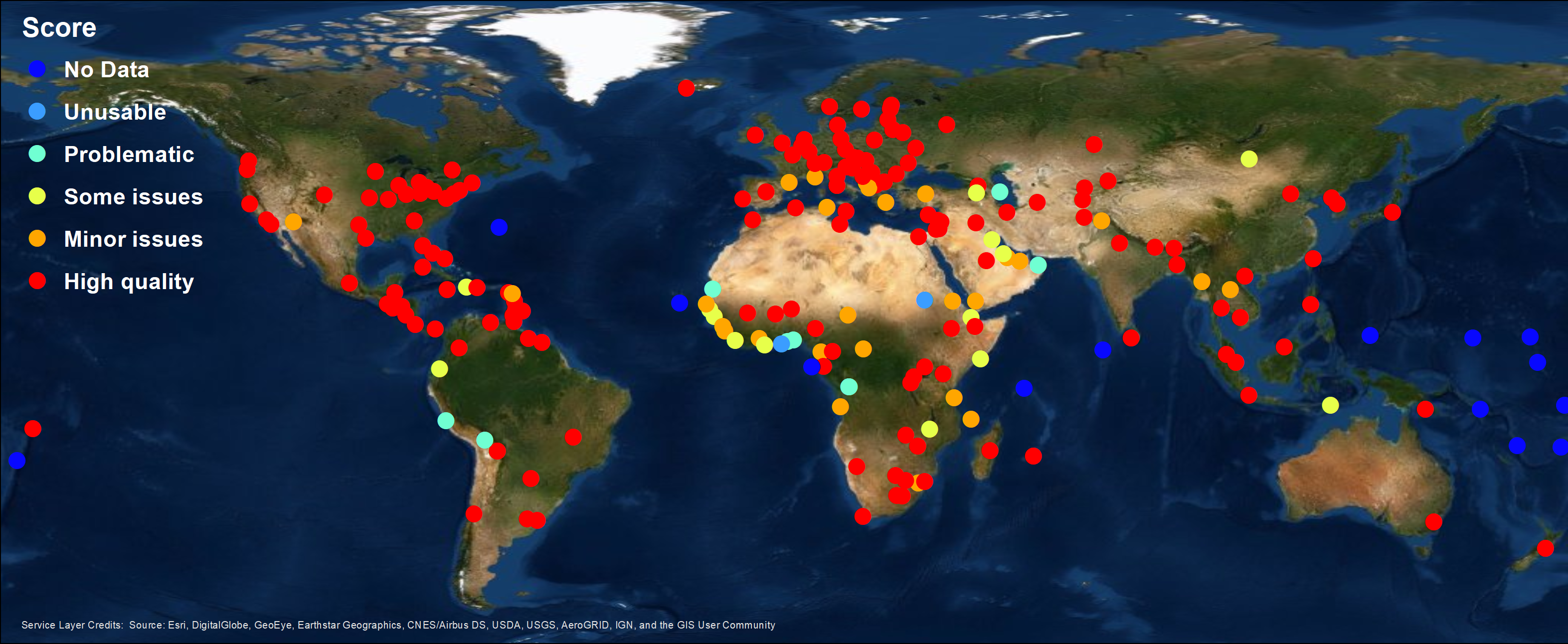
Figure 7: After testing in 224 large cities around the globe, the results show that for 83% of the cities assessed Trends.Earth data can be used for estimating indicator SDG 11.3.1. The biggest limitation remains in small island states (for which no training data was available), hyper arid areas, and areas with low image availability.
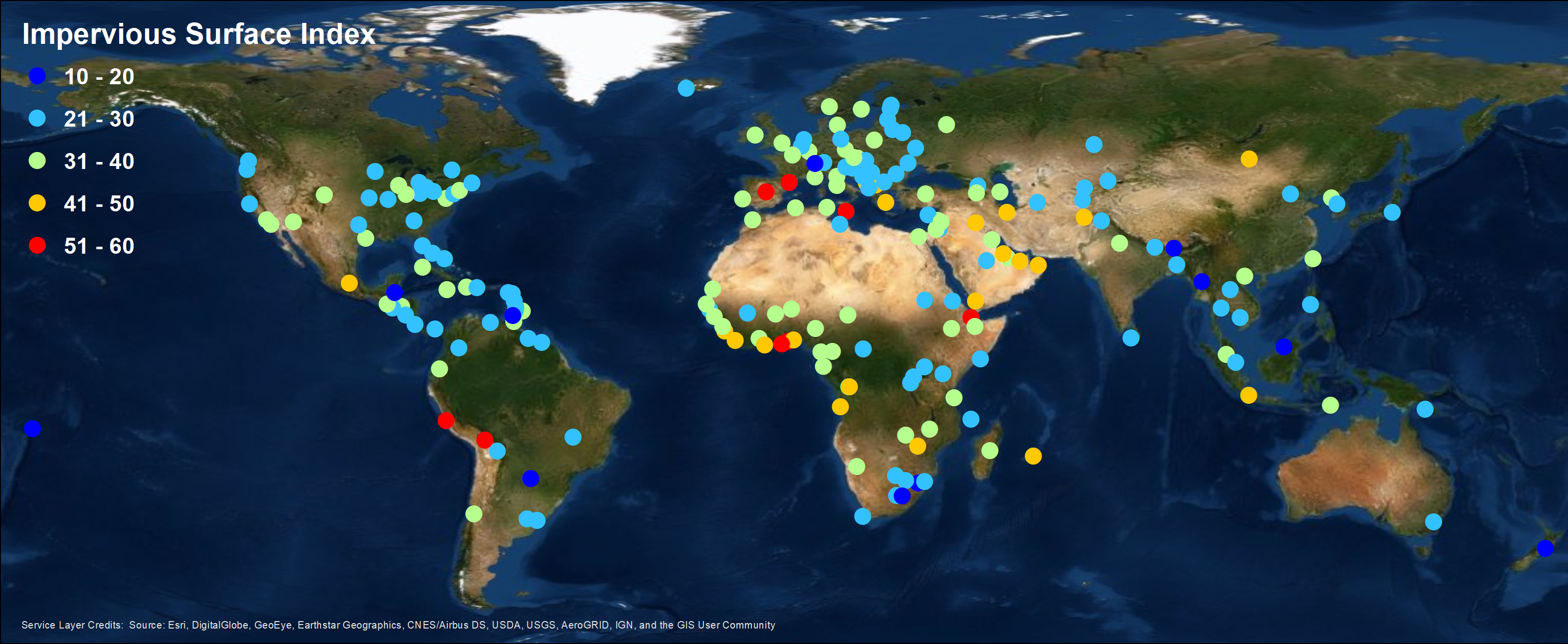
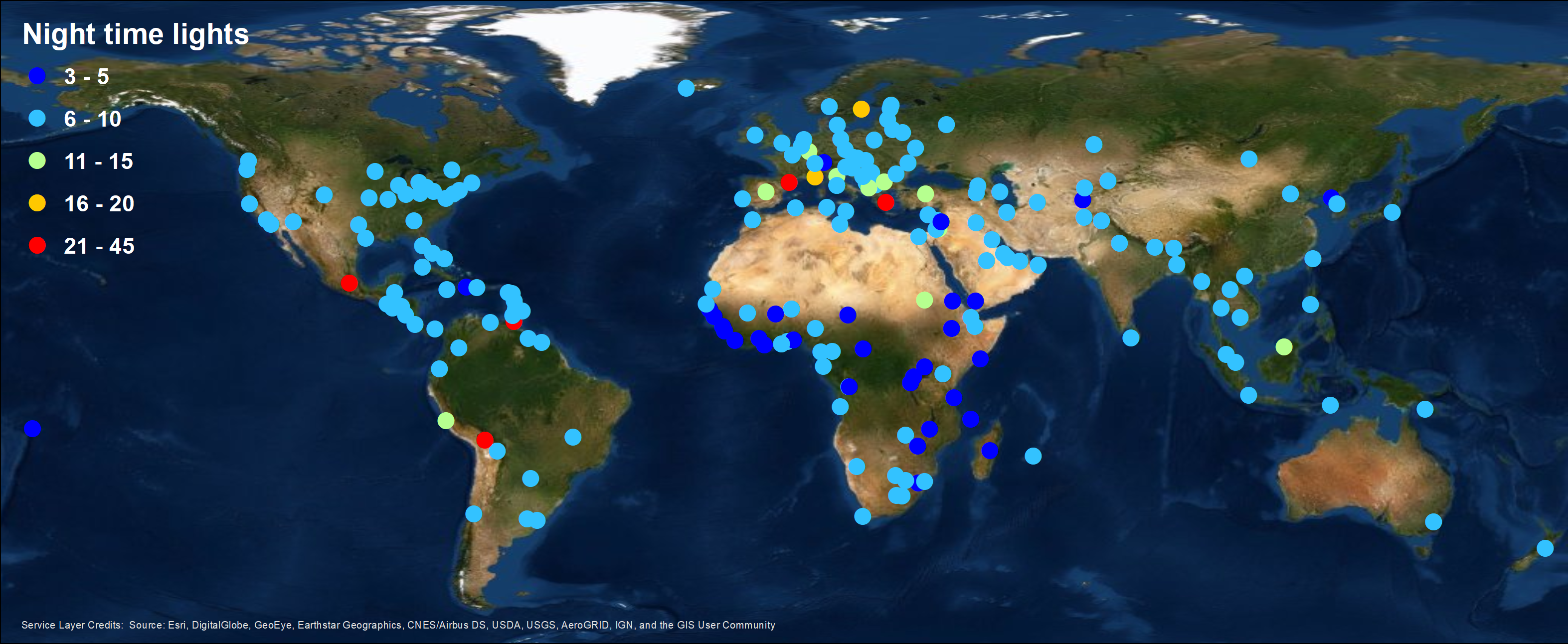
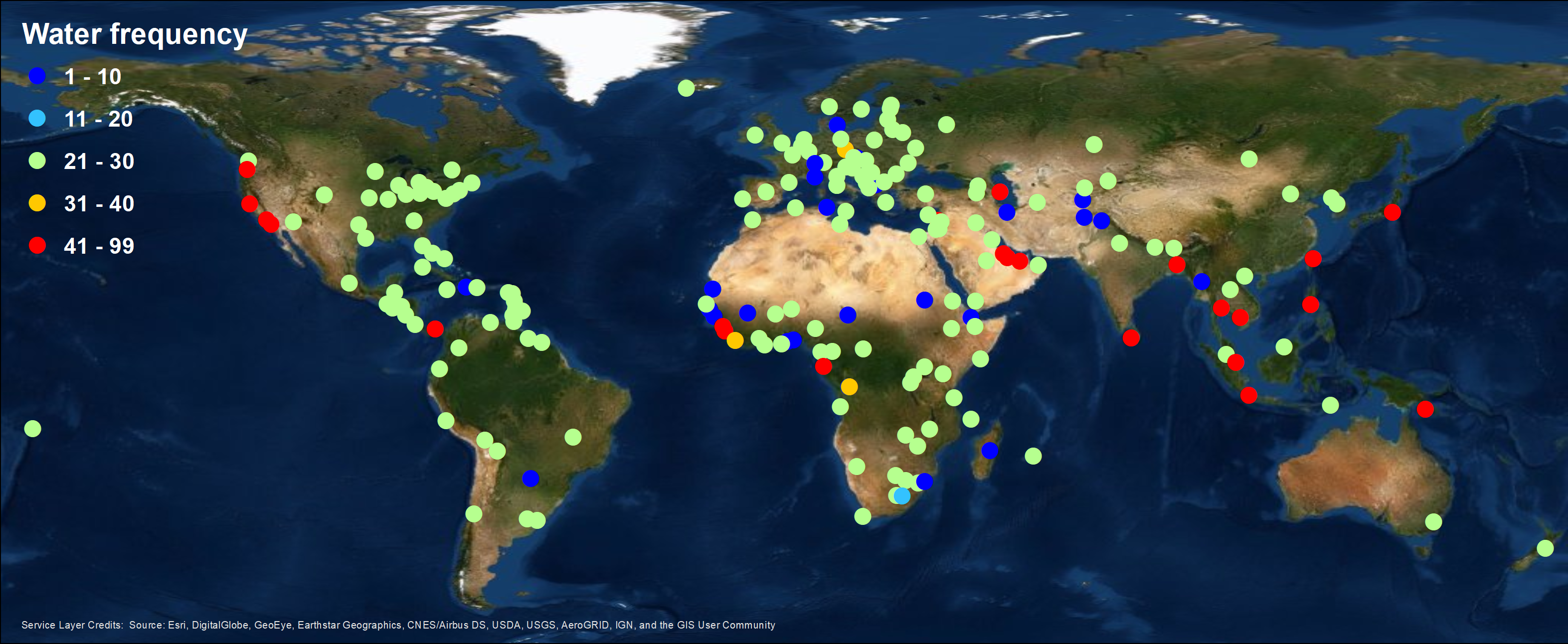
Figure 8: Spatial distribution of threshold parameters selected for the sample of 224 cities tested. Top: Impervious surface area indicator, Middle: Nighttime lights indicator, and Bottom: Water frequency indicator.
From the analysis of 224 cities globally we were able to estimate the range of parameters most commonly used. The most frequent values used were: ISI = 30, NTL = 10, WFR = 25. Those were the default parameters defined in the Trends.Earth Urban Mapper and QGIS plugin, but it is important to remember that for each city, careful inspection of the dataset should be perform, in order to find the set of parameters which better work for each site.
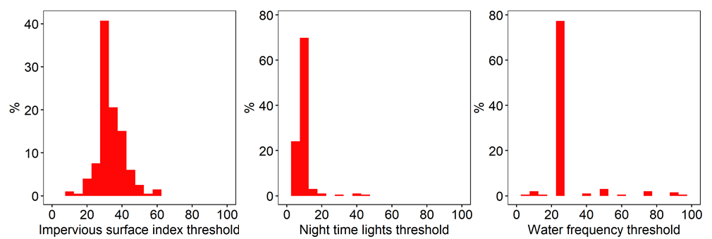
Figure 9: Frequency distribution of threshold parameters selected for the sample of 224 cities tested. Left: Impervious surface area indicator, Middle: Nighttime lights indicator, and Right: Water frequency indicator.
Urban zones
The urban extent is the proposed area of study that comprises of the built-up area and urbanized open space of the city, along with areas added by proximity analysis (UN-Habitat, 2019). UN-Habitat suggests classifying the area of interest into the 6 following classes in order to identify the area which will be used in the estimation of the annual land consumption rate (Figure 1):
Built-up areas will be classified based on the density within a 500 m of each pixel radius:
Urban: > 50% built-up in the 500 m radius.
Suburban: 25-50% built-up in the 500 m radius.
Rural: < 25 % built-up in the 500 m radius.
The non-built up areas will be considered open space (OS), and will be classified as follows:
Fringe open space: open space < 100 m from urban and suburban.
Captured open space: open space fully surrounded by fringe open space.
Rural open space: All other open space.
In ![]() , we have added to the scheme above by differentiating land from water open space, since the uses citizens can do of each space are very different.
, we have added to the scheme above by differentiating land from water open space, since the uses citizens can do of each space are very different.
Fringe open space - water: Fringe open space covered by water
Captured open space - water: Captured open space covered by water
Rural open space - water: Rural open space covered by water
Urban extent is determined by the combined area of classes 1, 2, 4, 5, 7, and 8 (urban, suburban, and fringe and captured open space).
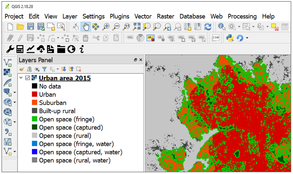
Figure 10: Result of the SDG 11.3.1 analysis displaying the different elements which comprise the urban space.
With this information we can now estimate the rates of urban expansion over time for the periods 2000-2005, 2010, and 2010-2015 needed to estimate the annual land consumption rate.
Population growth
Note
Source: UN-Habitat (2019) SDG Indicator 11.3.1 Training Module: Land Use Efficiency. United Nations Human Settlement Programme (UN-Habitat), Nairobi.
Once the urbanized areas have been defined, the next step is to establish how many people live within those areas for each analysis year. This information is then used to compute the annualized population growth rate. The estimation of the number of people living within each service area can be achieved through two broad approaches:
Use of high-resolution data from national statistical offices (NSOs): In this option, census data is used to aggregate the number of people living in all households within the urban boundaries. Projections and extrapolations can also be easily undertaken based on the household characteristics to particular reporting years. The process is much easier where dynamic census units are used to identify the urbanized area, particularly because these are well aligned with the official population data architecture. This option provides the most accurate and authoritative population data for the indicator computation and is highly encouraged.
Use of gridded population: In this option, a population grid is made by distributing population to the entire administrative or census area unit. Attributes such as presence of habitable areas (land use classes) can be used to distribute the population, such that grid cells in tracks of undeveloped land or in industrial areas will have less population than high density residential areas. In the resulting grid, each grid cell will have a unique value, which is dependent on factors such as the total population within the enclosing administrative/census unit, and the number and/or quantity of the habitable land use classes. Figure 5 illustrates the general logic of population grids using only one land use class – the built-up areas. The population grid should always cover an area larger than the defined urban boundaries. Once the population grids are created, estimation of the population living within the urban boundaries can then be achieved by aggregating populations of the enclosed grid cells. In the absence of high-resolution data from NSOs, this option produces better estimates for population, although high quality input data and multi-level analysis are essential for enhanced data accuracy. Global datasets representing populations at 1km² and 250m grids are available (e.gs GPWv4, GHS-POP, WorldPop); most of which assume equal distribution of population to the habitable classes (e.g built up areas). This approach is proposed for the indicator computation where high resolution data from national statistical offices is not available or readily accessible.
Population in Trends.Earth
In ![]() we recommend users to use option 1, since ate city scales the accuracy of high-resolution data provided by national statistical offices will always be higher than those obtained by global raster products which were, in most cases, produced for national level analysis. However, recognizing that in some areas population data will not be readily available to most users, we do provide data from the Gridded Population of the World V4 (GPWv4, CIESIN, 2016) as a reference. Even if the option to use GPWv4 in
we recommend users to use option 1, since ate city scales the accuracy of high-resolution data provided by national statistical offices will always be higher than those obtained by global raster products which were, in most cases, produced for national level analysis. However, recognizing that in some areas population data will not be readily available to most users, we do provide data from the Gridded Population of the World V4 (GPWv4, CIESIN, 2016) as a reference. Even if the option to use GPWv4 in ![]() , the population data can be easily replaced by locally relevant high quality data by simply replacing the corresponding cells in the final tabular output.
, the population data can be easily replaced by locally relevant high quality data by simply replacing the corresponding cells in the final tabular output.
Trends in SDG 11.3.1
The final outputs of the SDG 11.3.1 computations in ![]() will be:
will be:
The maps as presented Figures 10 and 11, which will allow for a visual interpretation of the changes occurred in the urban space between 2000 and 2015 at 5-year intervals.
A table which summarizes the area calculations for the different spaces within the city space (urban, suburban, and the different classes of open space), and also the corresponding population numbers. In this table the SDG 11.3.1 will also be computed automatically, and a trend of the indicator over time will be provided.
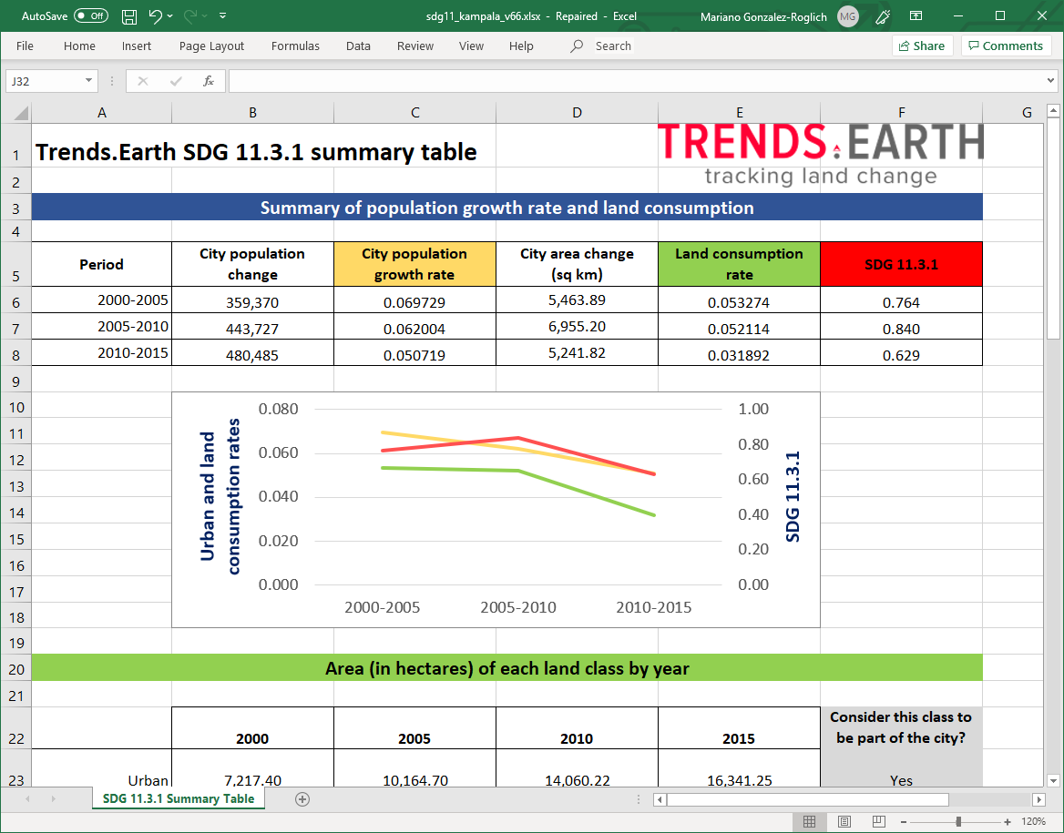
Figure 11: One of the final outputs of the SDG 11.3.1 analysis in |trends.earth| is a tabular outputs displaying the area, population and the indicator for SDG 11.3.1 for the city analyzed.
Note
For a step-by-step guide on how to run the analysis in ![]() , please refer to the following tutorial: Land Consumption (SDG 11.3.1).
, please refer to the following tutorial: Land Consumption (SDG 11.3.1).
Citations:
Breiman, L., 2001. Random forests. Mach. Learn. 45, 5–32. https://doi.org/10.1023/a:1010933404324
Brown de Colstoun, E. C., C. Huang, P. Wang, J. C. Tilton, B. Tan, J. Phillips, S. Niemczura, P.-Y. Ling, and R. E. Wolfe. 2017. Global Man-made Impervious Surface (GMIS) Dataset From Landsat. Palisades, NY: NASA Socioeconomic Data and Applications Center (SEDAC). https://doi.org/10.7927/H4P55KKF.
CIESIN. 2016. Gridded Population of the World, Version 4 (GPWv4): Population Density Adjusted to Match 2015 Revision of UN WPP Country Totals. Palisades, NY: NASA Socioeconomic Data and Applications Center (SEDAC). Center for International Earth Science Information Network - Columbia University. https://doi.org/10.7927/H4HX19NJ.
Dinerstein, E., Olson, et al, 2017. An Ecoregion-Based Approach to Protecting Half the Terrestrial Realm. BioScience 67, 534–545. https://doi.org/10.1093/biosci/bix014
Gorelick, N., Hancher, M., Dixon, M., Ilyushchenko, S., Thau, D., Moore, R., 2017. Google Earth Engine: Planetary-scale geospatial analysis for everyone. Remote Sens. Environ., Big Remotely Sensed Data: tools, applications and experiences 202, 18–27. https://doi.org/10.1016/j.rse.2017.06.031
Jean-Francois Pekel, Andrew Cottam, Noel Gorelick, Alan S. Belward, High-resolution mapping of global surface water and its long-term changes. Nature 540, 418-422 (2016). https://doi.org/10.1038/nature20584.
NOA. 2019. VIIRS Nighttime Day/Night Band Composites Version 1. Available through: https://developers.google.com/earth-engine/datasets/catalog/NOAA_VIIRS_DNB_MONTHLY_V1_VCMCFG
UN-Habitat (2019) Module 3: Land consumption. Accessed on 05/10/2019 from: https://unhabitat.org/wp-content/uploads/2019/02/Indicator-11.3.1-Training-Module_Land-Consumption_Jan-2019.pdf